XLOOKUP for Dummies – 4 Easy Examples
(Note: This XLOOKUP in Excel tutorial is suitable for users of Microsoft 365.)
In this guide, learn how to easily use XLOOKUP in Excel. XLOOKUP looks for a search term in one column and return the result from the same row in another column. But, unlike VLOOKUP, it can search for the values in all directions (top to bottom , bottom to top, left to right and right to left).
You’ll learn:
The XLOOKUP Function in Excel
XLOOKUP is a new lookup function in Excel. If you have ever used (and struggled with) INDEX and MATCH or VLOOKUP to perform complex lookups, then XLOOKUP is a notable alternative solution.
Use the XLOOKUP function when you need to find something in a table or range by row. For example, look up a product using the product ID, or find the price of a trip using the trip code.
XLOOKUP’s power comes from being able to look in one column for a search term and return the result from the same row in another column.
XLOOKUP is more flexible than other popular lookup functions like VLOOKUP. VLOOKUP limits you to only being able to find something in a table or cell range that is in a column to the right of the search term. XLOOKUP can return results no matter where they are in relation to the search term.
In this example, I have used XLOOKUP to return the ‘Category’, ‘Revenue’, and ‘Profit’ from the table for the ‘App’ shown in cell H3.


How to Use XLOOKUP in Excel?
Let us look at a basic XLOOKUP formula in action.
Example 1 – Simple XLOOKUP
This example uses a simple XLOOKUP to look up an ‘App’ name and return its ‘Category’, ‘Revenue’ and ‘Profit’.


Syntax
=XLOOKUP(lookup_value, lookup_array, return_array, [if_not_found], [match_mode], [search_mode])
| lookup | The cell that contains the lookup value, in this case H3 |
| lookup_array | The cell range where the lookup value is located, B4:B11 |
| return_array | The cell range that contains the information you want to return, A4:A11 |
This basic XLOOKUP formula does not include the optional arguments if_not_found, match_mode, and search-mode.
We are using the cell reference, H3 to specify the lookup value in the formula. If I type ‘Spotify’ into cell H3, the formula works, and I see the correct results.


Example 2 – XLOOKUP to Return Multiple Values
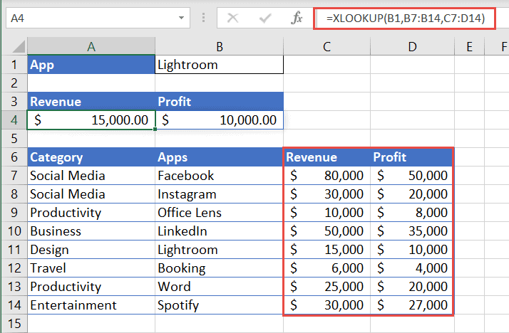
In this example, we are looking up the ‘Revenue’ and ‘Profit’ based on the ‘App’ in cell B1. Unlike VLOOKUP, XLOOKUP can return an array with multiple items, which allows a single formula to return both the revenue and profit from cells C7:D14


Example 3 – XLOOKUP to Return an ‘If not found’ Message
This example adds the if_not_found argument to the end of the previous example. In cell B1, the application name has a spelling error and so XLOOKUP returns the message ‘App Not Found’.


Example 4 – How to Use Named Ranges in XLOOKUP?
It is good to get into the habit of naming cell ranges. When you name a range, it gives meaning and helps others understand what cells you are referring to in formulas.
Naming a Range
- Select the cell range you wish to name
- In the Name box above, type in a meaningful name for the range
- Press Enter


The named ranges can now be used in the XLOOKUP formula instead of the cell ranges.


For further guidance on XLOOKUP, including more complex examples, check out the following links:
OR, if you are using Google Sheets. Take a look at Alternatives to XLOOKUP in Google Sheets.
XLOOKUP in Excel – Video Tutorial
To see XLOOKUP in action, please watch the following video tutorial.
How to Use XLOOKUP in Excel (13:45)
For more Free Excel tutorials from Simon Sez IT. Take a look at our Excel Resource Center.
To learn Excel with Simon Sez IT. Take a look at the Excel courses we have available.

