Creating a Dynamic Pivot Chart Title Based on Slicer(6 Easy Steps)

This Dynamic Pivot Chart Title tutorial is suitable for users of Excel 2013/2016/2019 and Excel for Microsoft Office 365.    

Objective 

Create a dynamic Pivot Chart title using the new TEXTJOIN function that changes depending on the selection made in the slicer.  

In this tutorial I’ll cover:

1. What is a Dynamic Pivot Chart Title? 
2. Video Tutorial – Pivot Chart Title Based on Slicer
3. How to Create a Dynamic Pivot Chart Title Based on a Slicer? 
4. Let’s Wrapup

Related:

How to Enable Excel Dark Mode? 3 Simple Steps

How to Add Error Bars in Excel? 7 Best Methods

How to Superscript in Excel? (9 Best Methods)

What is a Dynamic Pivot Chart Title? 

A dynamic Pivot Chart title is a title that changes based on the selection you have made.  

For example, if you have a Pivot Chart that is filtered using a slicer, you may want the pivot chart dynamic title to display the selection from the slicer. The title will change each time you make a new slicer selection making it easier to understand the data that is currently displayed.  

In this example, I have a PivotTable showing the total sales across different categories of products and a Pivot Chart that visualizes the analysis. I also have a slicer to filter the data by store.  

The Pivot Chart currently has a static title labelled ‘Sales by Category‘.

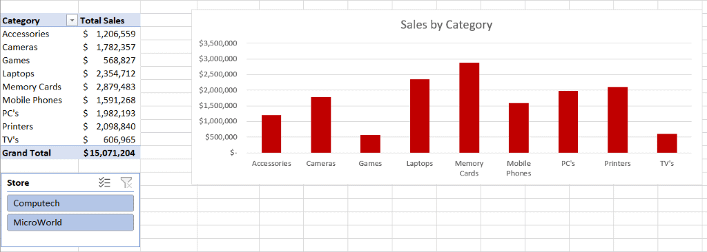
I want the title to reflect the current slicer selection. If ‘Computech’ is chosen in the slicer, I would like the chart title to say, ‘Sales by Store – Computech,’ and if ‘MicroWorld’ is selected, ‘Sales by Store – MicroWorld.’ If both stores are selected, I would like the chart title to reflect that.  

The process of making a chart label dynamic involves a few different steps. The method I am using in this tutorial is just one of the ways this can be achieved.

Video Tutorial – Pivot Chart Title Based on Slicer

To see Dynamic Labels in action, please watch the following video tutorial.  

Also Read:

How to Use the Excel Fill Handle Easily? (Top 3 Uses with Examples)

How to Shade Every Other Row in Excel? (5 Best Methods)

VLOOKUP for Dummies (or newbies)

How to Create a Dynamic Pivot Chart Title Based on a Slicer? 

Step 1 : Prepare your Data

As we are going to be performing a few different steps to create the dynamic chart title, I find it useful to create a ‘Helper’ worksheet to separate the calculations from the data.  

1. From the ‘Sales by Category’ worksheet, Cut (ctrl+x) the slicer 

2. Paste (ctrl+v) the slicer onto the ‘Helper’ worksheet 

 Next, I am going to create another PivotTable on the ‘Helper’ worksheet using the source data on the ‘Data’ worksheet.  

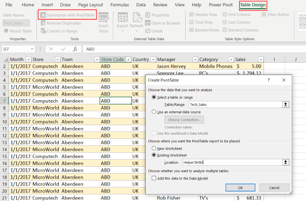
3. Drag the field used in the slicer, in this case, ‘Store’ to the Columns area 

4. Turn off Grand Totals for the PivotTable 

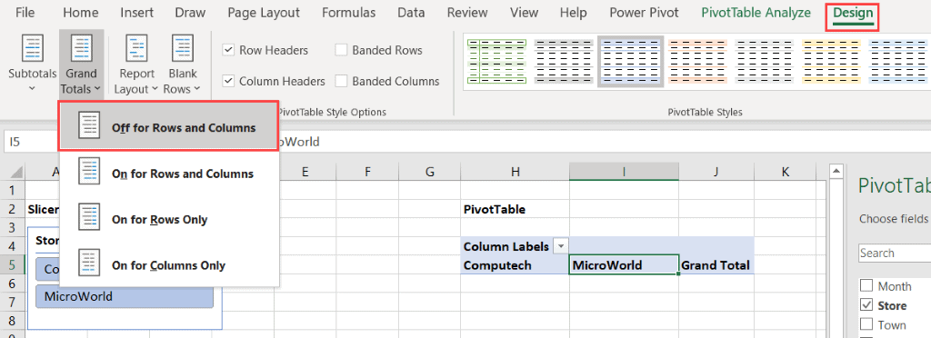
Everything is now in place to create the formula for the dynamic chart title.  

Step 2 : Create the Dynamic Pivot Chart Title 

1. On the ‘Helper’ worksheet, type the main title for the Pivot Chart 

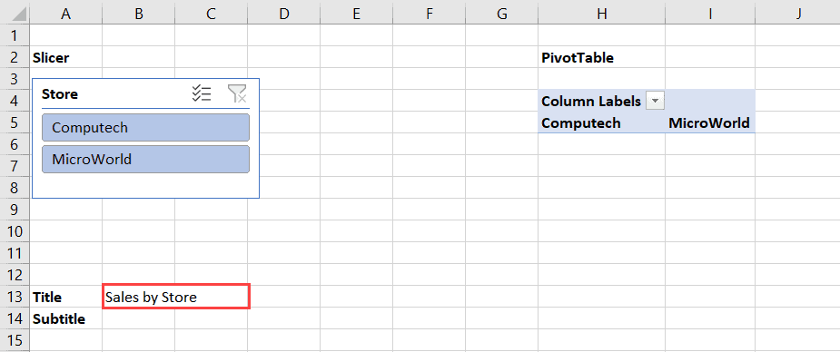
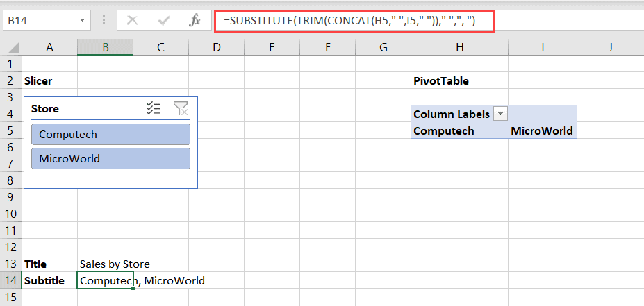
The subtitle will contain whichever store or stores we select in the slicer.  

For this, we need to use a formula. 

For Excel 2019/365 Users Only 

If you have 2019, 365, or a later version of Excel, you will be able to utilize the new TEXTJOIN function to construct the subtitle.  

This function has 3 arguments; delimiter, ignore_empty and text 

The delimiter tells Excel how you would like the words in the subtitle to be separated, in this case, with a comma. The TRUE argument tells Excel to ignore empty cells in the selection, which is row 5.  

For Excel 2010/2013/2016 Users 

If you are using an older version of Excel, you will not be able to use the TEXTJOIN function. Instead, you will need to use a combination of CONCAT or CONCATENATE, SUBSTITUTE, and TRIM to achieve the same result.  

Step 3: Connect the Slicer to the PivotTable 

The next step is to connect the slicer to the PivotTable on the ‘Helper’ worksheet.  

1. Select the slicer 

2. From the Slicer tab, in the Slicer group, click Report Connections 

3. Put a tick in the box next to the relevant PivotTable 

4. Click OK 

Test out the slicer. The subtitle and PivotTable should change according to the selection in the slicer.  

Step 5: Connecting the Dynamic Titles to the Pivot Chart 

The final step in the process is to connect the title and the subtitle to the Pivot Chart.  

1. Select the text box that contains the chart title 

2. In the formula bar, type = 

3. Click the ‘Helper’ worksheet and select the cell that contains the title ‘Sales by Store’ 

4. Press Enter 

5. From the Insert tab, in the Text group, select Text Box 

6. Draw a text box on the chart 

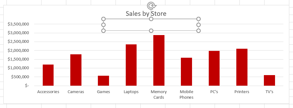
7. With the text box selected, type = in the formula bar 

8. Click the ‘Helper’ worksheet and select the cell that contains the subtitle  

9. Press Enter 

10. Format the chart title as desired 

11. Copy the slicer back to the ‘Sales’ worksheet and test it out 

Suggested Reads:

How to Group Worksheets in Excel? (In 3 Simple Steps)

Easily Make a Bullet Chart in Excel—2 Examples

How to Easily Create an Excel Histogram?—2 Best Methods

Let’s Wrapup

In this tutorial, I have covered the easiest method to add a dynamic pivot chart title based on a slicer. There are so many different methods and techniques for creating dynamic labels for charts and Pivot Charts. To see more of them, check out the links below.  

Trump Excel – How to Create Dynamic Chart Titles in Excel 

Dummies – The Art of Dynamic Labeling in Excel 

For more Free Excel tutorials from Simon Sez IT. Take a look at our Excel Resource Center.

Other Excel classes you might like:

• Dashboard in Excel Using Pivot Tables, Pivot Charts and Slicers
• Logical Functions in Excel
• Designing Better Spreadsheets in Excel
• Introduction to Power Pivot & Power Query in Excel

To learn Excel with Simon Sez IT. Take a look at the Excel courses we have available.

Deborah Ashby

Deborah Ashby is a TAP Accredited IT Trainer, specializing in the design, delivery, and facilitation of Microsoft courses both online and in the classroom.She has over 11 years of IT Training Experience and 24 years in the IT Industry. To date, she's trained over 10,000 people in the UK and overseas at companies such as HMRC, the Metropolitan Police, Parliament, SKY, Microsoft, Kew Gardens, Norton Rose Fulbright LLP.She's a qualified MOS Master for 2010, 2013, and 2016 editions of Microsoft Office and is COLF and TAP Accredited and a member of The British Learning Institute.