The Excel CHOOSE Function – 4 Best Uses

Note: This tutorial on the Excel CHOOSE function is suitable for all Excel versions including Office 365. 

The CHOOSE function is one of the most versatile tools available in Excel. When combined with other functions, it can solve challenging problems in innovative ways. 

In this guide, I’ll explain how to use the CHOOSE function along with some interesting ways of using it. 

Related:

How to Extract an Excel Substring? – 6 Best Methods

How to Superscript in Excel? (9 Best Methods)

How To Find Duplicates in Excel? (3 Easy Methods)

Excel CHOOSE Function – Overview

The CHOOSE function simply returns a value from a list based on a user-specified position in that list. 

For example,

=CHOOSE(2, "Alpha","Beta","Gamma") 

will return the value “Beta” as it is in the second position in that list. 

In other words, use it to get a value from a list based on its position in the list. 

Excel CHOOSE Function – Syntax

The CHOOSE function has the following syntax: 

=CHOOSE(index_num, value1, [value2], …)

Where index_num is the index number of the value in the list. That is the position of the value in the list. 

“value1, value2 …..” can be a  list of 254 values. Value1 is required and the rest are optional. These values can be direct numbers, direct text strings, cell references, formulas, or defined ranges. 

Also Read:

How to Use Goal Seek in Excel? (3 Simple Examples)

How to Insert Multiple Rows in Excel? The 4 Best Methods

How to Autofit Excel Cells? 3 Best Methods

How to use the Excel CHOOSE Function? 

As discussed earlier, the CHOOSE function becomes immensely useful when used in combination with other functions or features. 

In the following examples, I’ll explain how to use the CHOOSE function to make other functions more effective or to find simple solutions to complex problems. 

Replace Nested IFs with Excel CHOOSE Function

Let’s suppose you have to assign grades to students based on their marks, like this: A for marks 90 and above, B for marks 80-89, C for marks 70-79, and D for the rest. 

One way to do this is to use nested IF functions. But it is not a very user-friendly way to do it. 

The CHOOSE function is a much simpler alternative in these cases. 

=CHOOSE((B2>0) + (B2>=70) + (B2>=80) + (B2>=90), "D", "C", "B", "A")

Here, the index_num argument is (B2>0) + (B2>=70) + (B2>=80) + (B2>=90). What it does is that it checks for each condition and returns TRUE or FALSE.

Which in turn gets converted into 1 or 0 inside the formula. 

Hence, for cell B3 it looks something like this =CHOOSE(TRUE+ TRUE + FALSE +FALSE , “D”, “C”, “B”, “A”). 

Which further breaks down into =CHOOSE(1+ 1 + 0 +0 , “D”, “C”, “B”, “A”). 

This is nothing but =CHOOSE(2, “D”, “C”, “B”, “A”), which returns an answer “C” as the grade. 

Note that, you can use the cell references for the values list as well. For example, use =CHOOSE(1+ 1 + 0 +0 , $E$2:$E$5) instead of =CHOOSE(1+ 1 + 0 +0 , “D”, “C”, “B”, “A”).

Also, it is a good idea to wrap the CHOOSE function in IFERROR to avoid #VALUE errors, which might appear in case if there is not even one TRUE value. 

Use the Excel CHOOSE Function for a left VLOOKUP

The VLOOKUP function in Excel can only be used to return values to the right of the lookup column by default. But there is a simple trick to make VLOOKUP search to its left side, which involves the CHOOSE function. 

For example, here I have a list of product sales revenue followed by product names. If I directly use the VLOOKUP to look up the product name and return its corresponding revenue, it will return an error. This is because the return value is to the left of the lookup column. 

But, we can trick VLOOKUP into thinking that column B is the first column and column A is the second column. 

To do this, use =CHOOSE({1,2}, B2:B5, A2:A5) in place of the table_array argument inside the VLOOKUP function. So, the entire VLOOKUP formula will look something like this :

=VLOOKUP(E2,CHOOSE({1,2}, B2:B5, A2:A5),2,FALSE)

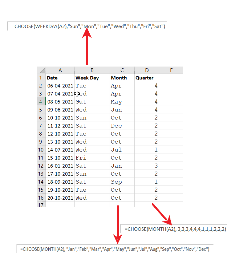
Use the CHOOSE Function to Assign Day/Month/Quarter to Dates

Let’s say you have a worksheet where you need to assign a custom day or month or quarter to your dates. You can do this easily using the CHOOSE function. Let’s see how. 

To assign Day names to your dates use: 

=CHOOSE(WEEKDAY(A2),"Sun","Mon","Tue","Wed","Thu","Fri","Sat")

where you can replace the day names with custom names of your choice. 

To assign Month names to your dates use: 

=CHOOSE(MONTH(A2), "Jan","Feb","Mar","Apr","May","Jun","Jul","Aug","Sep","Oct","Nov","Dec")

where you can replace the month names with custom names of your choice. 

To assign Quarters to your dates use: 

=CHOOSE(MONTH(A2), 3,3,3,4,4,4,1,1,1,2,2,2)

Use the Excel CHOOSE Function to Calculate the SUM of a Selected Variable

Let’s suppose you have a sheet containing the sales data for different regions. Now you want a user-friendly way to find the total sales in each region at the click of a button. 

To do this use the CHOOSE function inside a SUM function like shown below. 

=SUM(CHOOSE(G4,C3:C5,D3:D5,E3:E5))

Here, the value in cell G4 acts as an index for the list of three ranges. The CHOOSE function returns the region list of your choice and lets the SUM function find its total. 

CHOOSE Function Excel Warnings and Errors

1. The CHOOSE function returns a VALUE! Error when the index_num is less than 1 or greater than the number of values in the list. 

2. It returns “#NAME?” error if the text strings in the list values are not enclosed in “quotes” or if the list reference is invalid. 

Suggested Reads:

How to Group Worksheets in Excel? (In 3 Simple Steps)

How to Shade Every Other Row in Excel? (5 Best Methods)

How to Use the Excel Fill Handle Easily? (Top 3 Uses with Examples)

Let’s Wrap Up

That’s all about the Excel CHOOSE function. If you have any questions about this or any other Excel feature, let us know in the comments. We are always happy to help. 

If you need more high-quality Excel guides, please check out our free Excel resources centre.

Ready to dive deep into Excel? Simon Sez IT has been teaching Excel for over ten years. For a low, monthly fee you can get access to 100+ IT training courses. Click here for advanced Excel courses with in-depth training modules.

Adam Lacey

Adam Lacey is an Excel enthusiast and online learning expert. He combines these two passions at Simon Sez IT where he wears a number of different hats.When Adam isn't fretting about site traffic or Pivot Tables, you'll find him on the tennis court or in the kitchen cooking up a storm.