6 Easy Methods to Strikethrough in Excel
Note: This tutorial on strikethrough in Excel is suitable for all Excel versions including Mac and Office 365.
Excel is a great program for crunching numbers and there is no doubt about that. However, when it comes to formatting text, it can be a little confusing if you are not already familiar with some of the features.
Strikethrough is one such example. We are sure you have frantically searched for the strikethrough option in the Excel ribbon but, to your disappointment, didn’t find it.
In this short guide, we will show you some easy methods to apply strikethrough in Excel.
You’ll learn:
Related:
Easily Make a Bullet Chart in Excel—2 Examples
Creating a Dynamic Pivot Chart Title Based on Slicer(6 Easy Steps)
How to Make a Line Graph in Excel? 4 Best Line Graph Examples
How to Apply Strikethrough in Excel?
Before we begin, let us first understand what strikethrough means. A strikethrough is just a line that crosses over the values of a cell. This is an example. It is a formatting style that is generally used to indicate edits, cancelled or completed items in a spreadsheet.
There are different ways to do this in Excel. Let us start with the easiest one.
Excel Strikethrough Keyboard Shortcut
The keyboard shortcut to apply strikethrough in Excel is Ctrl+5. You can apply it by selecting a single cell, parts of a single cell, or a range of cells. You can even select multiple non-adjacent cells by holding the Ctrl button and clicking them.
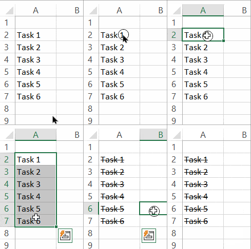

Once you have selected the required cells, just press the keyboard buttons Ctrl and 5 together. All your selected cells will be struck off by a single line.
How to Apply Strikethrough via Format Options?
Not a fan of shortcuts? Don’t worry, we’ve got you covered. You can still easily apply strikethrough using the Excel Format options.
Just follow these steps:
- Select the cells, part of cell or range of cells you want to be struck off.
- Right-click on your selection and click on Format Cells options. Alternatively, you can use the shortcut Ctrl+1.


- In the Format Options dialogue box, check the tick-mark next to the Strikethrough option in the Font section.
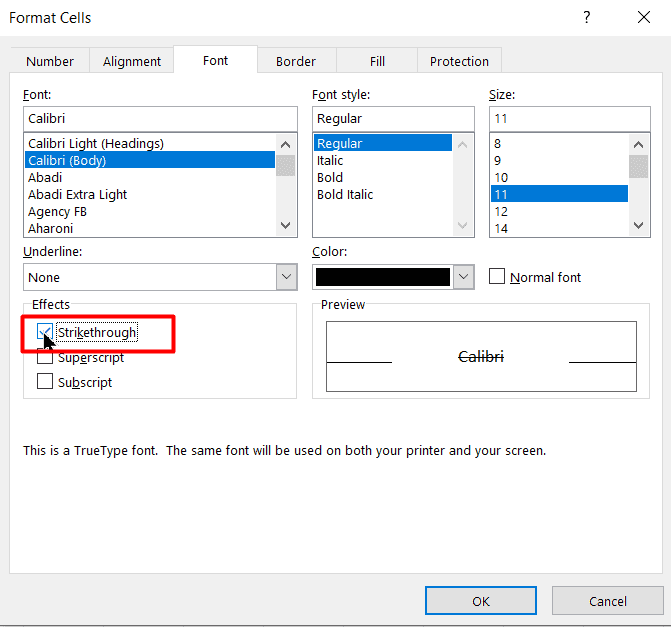

- Click OK.
How to Apply Strikethrough to Multiple Sheets using VBA?
All the methods that we just discussed apply to cells of a single sheet. In some cases, you may have too many cells that need to be striked off in one go. What if you need to strikethrough multiple cells split across multiple sheets? Don’t worry, as VBA codes come to your rescue.
First, select the cells you want to strikethrough across multiple sheets by holding down the Ctrl button.
Then run the following VBA code in the VBA editor ( Alt + F11)
Sub ApplyStrike()
Dim Ws As Worksheet
On Error Resume Next
For Each Ws In ActiveWorkbook.Worksheets
      Selection.Font.Strikethrough = True
      Next Ws
End Sub
This will apply the strikethrough formatting to all selected cells in that particular Excel workbook.
How to Apply Strikethrough on Excel Mac Version?
If you are using a Mac, you can easily apply a strikethrough to selected cells, using the shortcut Command + Shift + X.


Alternatively, you can use the same steps followed in the Format option method.
Also Read:
How to Use Goal Seek in Excel? (3 Simple Examples)
How to Insert Multiple Rows in Excel? The 4 Best Methods
How to Autofit Excel Cells? 3 Best Methods
Shortcut Buttons for Strikethrough in Excel
You can add a shortcut button to strikethrough text either in the quick access toolbar or the Excel ribbon. Here’s how:
Add a Strikethrough Shortcut Button in the Quick Access Toolbar
- Click on the drop-down button in the Quick Access toolbar and click on More Commands.


- In the Customise Quick Access toolbar menu, find and select the Strikethrough option from the Commands Not in the Ribbon section and click on the Add option.


- Click OK.
The Strikethrough option will now permanently appear in the quick access toolbar for your ease.


Add a Strikethrough Shortcut Button in the Excel Ribbon
If you are not very comfortable using the Quick Acess Toolbar, you can add a similar strikethrough shortcut button to the Excel Ribbon. Follow these steps:
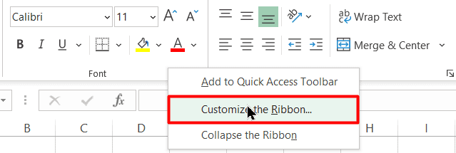
- Place your cursor anywhere on the ribbon and right-click on it.
- Click on the Customise Ribbon option from the right-click menu.

- In the Customise Ribbon menu click on any one of the target tabs on the right-hand side to a new group and rename it appropriately. In this example, I am using the one which I had already created for the subscript and superscript options.
- Select the newly created group.
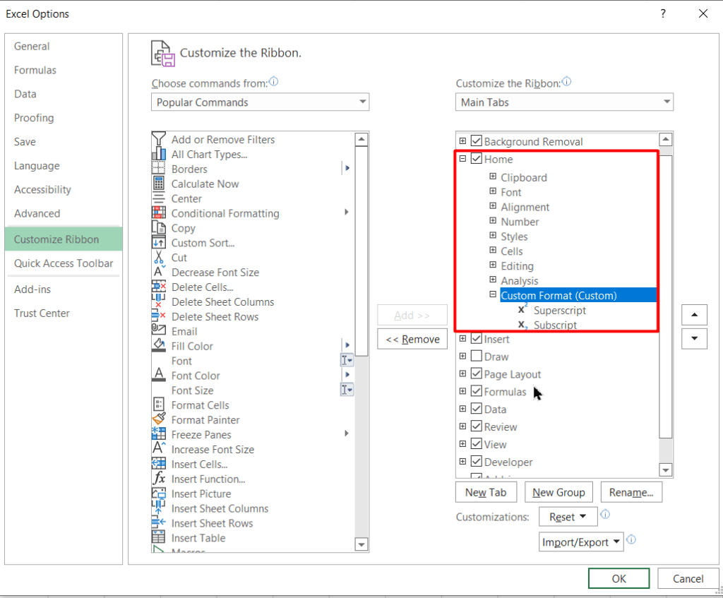

- Find and locate the Strikethrough option from the list on the left-hand side under the Commands Not in the Ribbon section.


- Click Add and Press OK.
This will insert a custom strikethrough option to the specific group in the Home tab. You can use it any time you want to apply the strikethrough format to your cells.


Suggested Reads:
How to Add a Watermark in Excel? 2 Easy Methods
How to Remove Hyperlinks in Excel? 3 Easy Methods
How to Use the Format Painter Excel Feature? — 3 Bonus Tips
Closing Thoughts
In this guide, we looked at how to easily apply a strikethrough in Excel, the easy way. We hope you found this guide helpful.
If you have any questions about this or any other Excel feature, please feel free to ask in the comments section.
Simon Sez IT has been teaching Excel for over ten years. For a low, monthly fee you can access over 100 IT training courses by seasoned professionals. Click here for advanced Excel courses with in-depth training modules.
Need more high-quality Excel guides? Check out our free Excel resources centre.

