How to Use Custom Number Formatting in Excel
(Note: Suitable for users of Excel 2013, 2016, 2019, 2021, and Excel for Microsoft 365.)
Objective
Understand how custom number formats work and how you can create your own custom number formatting.
Custom Number Formatting in Excel Explained
If you’ve been using Excel for a while, you are probably aware of how we can change the look of numbers in cells by applying number formatting.
Number formats control how numbers are displayed in Excel without changing the actual value. They are a quick way to apply formatting and make spreadsheets easier to read with a more consistent and professional look.
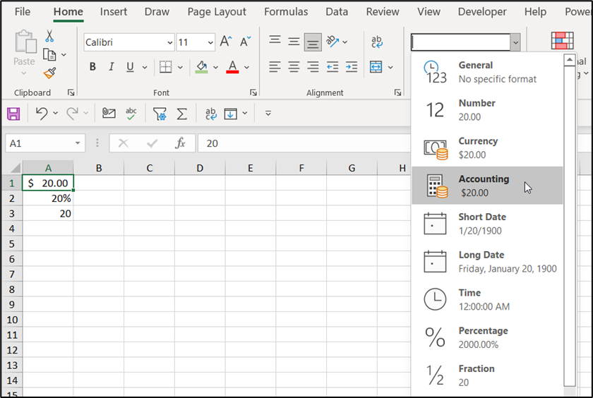
For example, we might want the value 20 to appear as $20 or 20%. We can apply simple number formatting to accomplish this.


There are numerous different number formats available in Excel: General, Number, Currency, Accounting, Short Data, Long Date, Time, Percentage, Fraction, Scientific, Text and Custom.
In this article, we are going to focus on Custom Number Formatting.
Using Custom Number Formats, we can be very specific about how we want to format values. For example, we might want to format dates in a spreadsheet to who the month names only or format very large numbers in millions. Maybe we want negative numbers to show in blue font.
We can do all of this with custom number formatting.
Related reads:
How to Use Excel MATCH Function
How to Graph a Function in Excel
How to Use SUMPRODUCT Function in Excel
Number Formatting
Number formatting controls how a value is displayed in Excel.
Let’s first understand how number formatting changes the output result for a date in a cell.
If we type the date, 10-Nov-2021, it is essentially formatted as dd-mmm-yyyy. We can modify this to change the look of the date.
| Date | Format | Output |
| 10-Nov-2021 | dddd | Thursday |
| 10-Nov-2021 | ddd | Thur |
| 10-Nov-2021 | dd | 11 |
| 10-Nov-2021 | mmmm | November |
| 10-Nov-2021 | mmm | Nov |
| 10-Nov-2021 | yyyy | 2021 |
| 10-Nov-2021 | yy | 21 |
Custom Number Formatting
Where to Find Custom Number Formatting
We can access Custom Number Formatting in two ways: from the ribbon or by using a keyboard shortcut.
From the Ribbon
- From the Home tab, in the Number group, click the drop-down next to General.
- Click More Number Formats.
- In the Format Cells dialogue box, click Custom.


Using a Keyboard Shortcut
We can access Custom Number Formatting using a keyboard shortcut.
- Press Ctrl+1.
- In the Format Cells dialogue box, click Custom.
Format Cells
In the Custom category of the Format Cells dialog box, we have a list of codes we can use to format our numbers, along with an input area to enter codes manually and a preview of the number.
In this example, I have 1567 in a cell. I can change the way this number looks by applying a different number format.


If we select a different code from the list, it will change the way the number looks in the preview.
Here, I’ve selected the #,##0 number format from the list of presets and it’s changed the number so there is a comma separator.


Aside from the preset formats, we can manually change the formatting by modifying the Type field.
Here, I’ve added a $ symbol in the Type field to change the value to a currency.


Suggested reads:
How to Create an Excel Gauge Chart the Easy Way
Battle of the Excel Lookup Functions: VLOOKUP vs INDEX/MATCH vs XLOOKUP
Custom Number Format Rule
We can format numbers quickly using one of the preset custom formats in the list.


It’s important to understand what we are looking at. There are 4 parts or sections to a Custom Number Format rule. Each part is separated with a semi-colon.
Part 1 – how to format a positive number
Part 2 – how to format a negative number
Part 3 – how to format zero values
Part 4 – how to format text
Positive;Negative;Zero;Text
In this example, we have the number 1567 in a cell. As it is a positive number, the formatting in Part 1 will be applied. The custom format we have selected from the list only formats positive numbers.


If we apply this format to the number, it will change to have two decimal places.


If we change the number to a negative number, -1567 and apply the custom formatting shown below, the formatting in part 2 will be applied as it’s a negative number. Notice here that positive numbers will be formatted with two decimal places, and negative numbers will show in red, in brackets and with two decimal places.


The result looks like this.


What about if we want negative numbers to show in Blue with no decimal places? We can edit the custom format.
In the Type field, we can change the word [Red] to [Blue] and remove the trailing zeros (00).


The result looks like this


Maybe I want zero values to show in red instead. We can edit the custom format. Remember, zero values are part 3.
Here, I’ve added another semi-colon and added the word [Red]. This is in position three so this formatting applies to cells that contain zero values.


This is the result.


Special Characters
We can utilize special characters when writing a Custom Number Format rule.
@ Symbol
The @ symbol controls where your text value shows up in your rule.
For example, maybe I want to format these text strings with the word ‘INV-‘ at the beginning to show they are invoice numbers. We can use the @ symbol to tell Excel where we want the invoice numbers to appear, in this case, after the specified text shown in quote marks.
Remember, part 4 of the custom format rule deals with text.


This is the result.


Comma Symbol
We can skip to the next part of the custom format rule using the comma symbol.
For example, maybe we want to format the number 10000000 as 10M.
The # symbol represents the first part of the number (10), then we have two commas. Effectively we are saying we require no specific format for negative numbers or zero values. However, we want to add the text “M” at the end.


This is the result.


Date and Time
We can apply the same principles when formatting other types of data. For example, date and time. We can choose a custom format from the preset list or we can construct our own if we want to be very specific.
Here I have selected a preset from the list that will change the format of the date from 12/1/2021 to Dec-21.


If we want to date to say Dec-2021 instead, we can edit the custom format.


Or we can build a new custom format if we need to be very specific.


Also read:
How to Password Protect an Excel File
How to Use the Excel IFS Function
Please visit our free resources center for more high-quality Excel and Microsoft Suite application guides.
Ready to dive deep into Excel? Click here for advanced Excel courses with in-depth training modules.
Simon Sez IT taught Excel and other business software for over ten years. You can access 150+ IT training courses for a low monthly fee.


