Dynamic Arrays: How to Use the Excel SEQUENCE Function and Unstacking Records
(Note: Suitable for users of Excel 2021 and Excel for Microsoft 365.)
Objective
Use the SEQUENCE Function to generate a list of sequential numbers in an array and see how the SEQUENCE Function can be combined with other Excel functions to provide practical solutions to common problems.
The SEQUENCE Function Explained
In its simplest form, the SEQUENCE function outputs a list of sequential numbers. We can specify how many rows and how many columns we need and also the step value.
The SEQUENCE function is one of the new dynamic array functions in Excel and so has the ability to ‘spill’ results into multiple cells.
SEQUENCE can be used on its own to produce a list of numbers or can be combined with other functions to perform more practical tasks.
The SEQUENCE function has 4 arguments, the last 3 are optional.
SEQUENCE(rows,[columns],[start],[step])
| rows | The number of rows of numbers required. |
| columns | The number of columns of numbers required. |
| start | The number to start at. |
| step | The interval between each number. create |
Related reads:
How to Use Excel MATCH Function
How to Graph a Function in Excel
How to Use SUMPRODUCT Function in Excel
Basic Example
In this example, we are going to generate a list of numbers 4 rows by 5 columns. We will start at 1 and the step value will be 1.
- Click on any cell in the worksheet
- Type =SEQUENCE(4,5,1,1)
The result is a table of numbers, 4 rows by 5 columns. The start value is 1 and each value increases by 1 each time (step).


Let’s modify the formula.
- Type =SEQUENCE(3,7,5,10)
The result is a table of numbers, 3 rows by 7 columns. The start value is 5 and each value increases by 10 each time (step).


Notice the result of this formula behaves like a dynamic array and ‘spills’ the results into other cells. It’s worth noting that to edit a dynamic array formula, we must be clicked in the original cell or the formula will be greyed out in the formula bar.


Practical Applications of SEQUENCE Function
Generating a Date Schedule
The ability to generate a list of numbers by specifying the rows, columns, start value and step value is reasonably useful in some situations but how can we really super-charge the SEQUENCE function and put it to good, practical use?
We could use the SEQUENCE function to help is generate a date schedule.
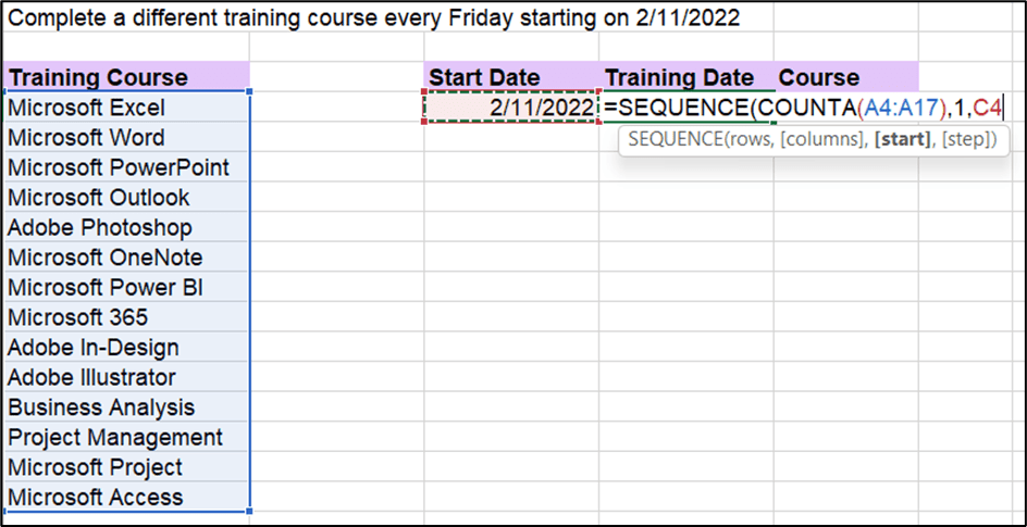
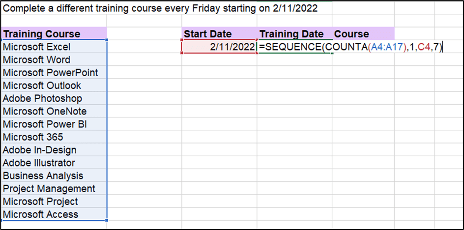
Here we have a list of training courses. It’s our 2022 goal to complete a different training course every Friday, starting on 2/11/2022. So, we want to list out the training dates and then assign courses to those training dates. We can use the SEQUENCE function to help us with this.


- Type =SEQUENCE
The number of rows is going to be the number of training courses we have in this list. We’re not going to manually count the entries, instead we are going to use the COUNTA function to do it for us. Remember, we need to use COUNTA and not COUNT if we are counting text.


Next, we specify the number of columns that we need. We are just filling training dates down, so I only need 1 column.


Now we need to specify the start value. The start value in this example, is the start date. As we have the start date in a cell, we can use the cell reference.


What will the step value be? Well, we want to complete a different course every Friday which is every 7 days. So, our step value will be 7. If we wanted to complete a course every 2 weeks, the step value would be 14.


Apply date number formatting to the results, if required.


Suggested reads:
How to Create an Excel Gauge Chart the Easy Way
Battle of the Excel Lookup Functions: VLOOKUP vs INDEX/MATCH vs XLOOKUP
Unstacking Records
We can also use the SEQUENCE command to take the hard work out of unstacking and organizing records in Excel.
What is unstacking? Let’s look at an example.
We have a list of training courses in column A. They are listed vertically by course name, level, location and date and that pattern repeats for all training courses. The layout of the list is not the easiest to read, so we would like to change the layout of the data, effectively unstacking the records into neat, vertical columns.


We also want this list to be dynamic so everything updates when a new course is added. To do this, we need to format our data as a table.
- Click in the data.
- Press CTRL+T.
- Click OK.


- Click in cell C4.
Type SEQUENCE and use COUNTA to find the number of rows required. Remember, we will see table references instead of cell references as we formatted our data as a table.


The number of columns we need to populate is 4 as we have 4 columns headings. We do not need to provide a start or step value.


The result, as you might expect is a large list of numbers. Each number relates to an item in column A. For example, 1 to 4 represents the course name, level, location and date for the first course in the list. 5 to 8 represents the information for the second course in the list, etc.


However, this pattern means we should have 24 courses. We don’t. We only have 6 courses in our list. So, we need to modify the formula and divide it by 4.


Now we have 6 courses represented by values. These are essentially the row numbers of the information they represent.


We can now use the INDEX function to return the correct results. Note the addition of the # (pound) symbol when the dynamic array is selected. This ensures the results will spill.


The records are now unstacked and organized into neat columns.


As we formatted our data as a table at the beginning, any new courses added to the list will dynamically update in the unstacked table.


Also read:
How to Password Protect an Excel File
How to Use the Excel IFS Function
Please visit our free resources center for more high-quality Excel and Microsoft Suite application guides.
Ready to dive deep into Excel? Click here for advanced Excel courses with in-depth training modules.
Simon Sez IT taught Excel and other business software for over ten years. You can access 150+ IT training courses for a low monthly fee.


