How to Use the Vertical Lookup Function in Excel 2016

In the previous section we examined Lookup Functions and their use within a horizontal list of values (HLOOKUP). Today we are going to examine a vertical list of values to lookup (VLOOKUP).

Their functions are similar in nature, the only difference being a vertical versus a horizontal lookup direction. However, we are also going to examine some more complex uses of the Lookup Function.

What is the Vertical Lookup Function?

The vertical lookup function is especially useful in the creation of an invoicing system. Let’s take a closer look on how the VLOOKUP function can be used to input details of a customer order and create an invoice.

How to Use the Vertical Lookup Function

In the body of the worksheet we will specify details such as the Quantity, Part Number, and Discount, and details such as Description, Unit Price, Discounted Price, and Total Price will automatically be specified.

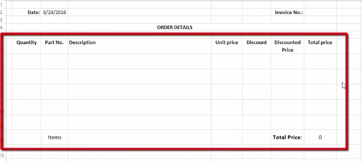
You may be wondering where this information will be pulled from. We already have a catalogue opened in sheet 2 of our Excel workbook.

Our catalogue contains details such as Part Number, Description, and Price.

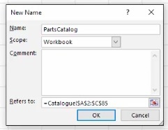
The very first thing that we want to do is define our List, or Catalogue, Name so that we may reference it in our invoice sheet.

1. Select all the values of the List
2. Select “Formulas” in the tool bar, then “Define Name”
3. Name your list in the dialogue that appears.
4. Set the Scope to Workbook (so that you may reference it in other sheets).

Now that this is set, we will return to our first sheet. Our first step in setting up the invoice is using the VLOOKUP function to render a description when we enter a Parts Number.

First, we will pull up the VLOOKUP function dialogue and specify our arguments.

• Our Lookup_value is the cell in which we will specify the Parts Number – C7.
• The Table_array is the list we are referencing – PartsCatalog
• The Col_index_number (column index number), is the column that we want to reference in our list. In this case, we want Column 2, or the Description column – 2.
• The Range_lookup refers to the values that are recognized and accepted in our formula. Since we are looking for an exact match, we will set this to FALSE.

Once our arguments have be inputted, we will get an error message of “#N/A” in the description box until we input a Part Number for the description to reference.

Repeat this process in the Price box using Column 3 from the catalogue list so that our product numbers will also render a price in our invoice.

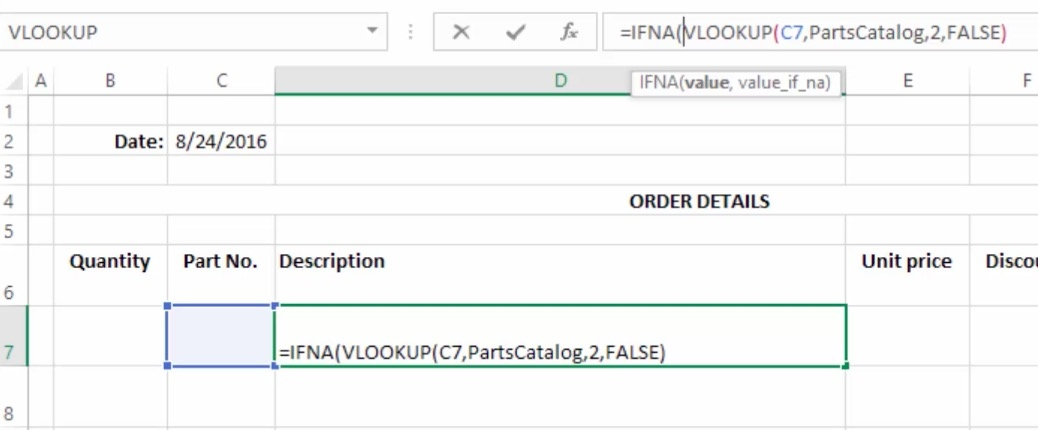
Removing the Error Message with the IF NA Function

Removing the error message or specifying a new message in the case of an error is simple.

1. Click on the description box that has the VLOOKUP function.
2. Add the term, IFNA, before the VLOOKUP formula.
3. Specify your error message following the VLOOKUP formula. If you want an empty cell in case of an error, specify a space as such: “ “

This entire cell formula will now look like this: IFNA(VLOOKUP(C7,PartsCatalog,2,FALSE), “ “)

This means that the cell will display a valid description unless an invalid product number (or no product number) is defined. In the case of NA, the cell will appear empty.

Get our complete Microsoft Excel 2016 training courses for beginner, intermediate and advanced learners. Click here to learn more. >>

Simon Calder

Chris “Simon” Calder was working as a Project Manager in IT for one of Los Angeles’ most prestigious cultural institutions, LACMA.He taught himself to use Microsoft Project from a giant textbook and hated every moment of it. Online learning was in its infancy then, but he spotted an opportunity and made an online MS Project course - the rest, as they say, is history!