Creating and Formatting Sparklines in Excel 2010
Synopsis: Sparklines were introduced in Excel 2010. In this article, we look at how to create and format these tiny charts.
Until now Excel charts have been graphic objects that are generally positioned and sized independently of worksheet cells. In Excel 2010 Microsoft introduced the Sparkline, a new type of chart that actually lives in a worksheet cell. They can be particularly useful when you are short of space, or when you need to give a simple graphical message without a lot of detail or artistic elaboration.
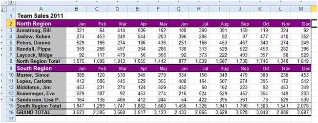
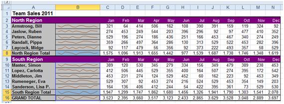
Look at this worksheet of sales data for 2011.
The monthly sales data for each member of a team is shown. We can look at the numbers for each team member but there is no simple visual snapshot of how each of them is doing, or of how the two sales regions are doing overall.
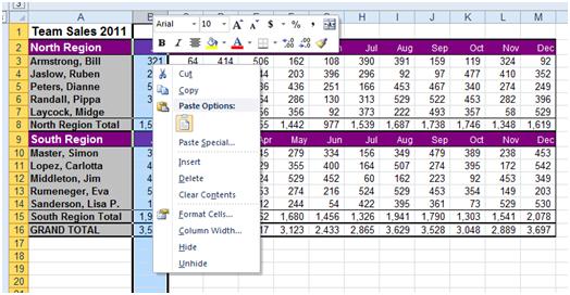
Let’s insert a new column before the January one and insert Sparklines to see how they look. First, select Column B and right click to see the shortcut menu.
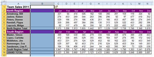
Select Insert, and Excel 2010 creates a new empty column.
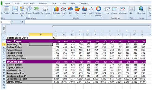
Select cell B3, then select the Insert tab. You should see the Sparklines group on the ribbon.
Click Line in the Sparklines group.
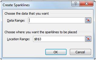
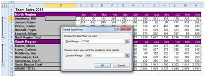
You use the Create Sparklines dialog first to choose the data to be reported on. There is no need to type into the Data Range box, although you can if you want to. Just select the cells to be reported on using the mouse as shown here.
The selected cells are surrounded by the “marching ants” selection box and the cell range is automatically shown in the Data Range box in the Create Sparklines dialog. In this case the range is “C3:N3”.
You can place the Sparkline in any worksheet cell, but Excel 2010 defaults to placing it in the cell you previously selected, which in this case is B3. That selection is shown in the Location Range box in the Create Sparklines dialog.
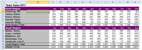
Click OK and the Sparkline is created.
Notice that in this case the Sparkline shows a slight deterioration in the sales person’s performance with strong seasonal variations as well.
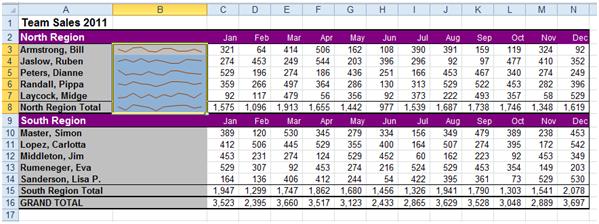
You don’t need to repeat this process for each of the other cells in Column B. You can copy and paste, or even use Fill Down. For example, select B3 then drag down with the mouse to B8. Then use the keyboard shortcut Ctrl-D to fill down.
Sparklines are created for each of the selected cells. (The Sparklines themselves are treated as a group in Excel, and if you want to work on them individually you will need to ungroup them.)
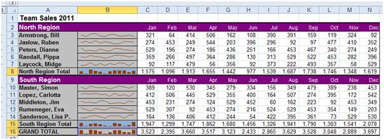
It’s easy to change the formatting of one or more Sparkline. Here I’ve selected the Sparklines for the two regional totals and the Grand Total.
Now, on the Design tab, in the Type group, select Column. The three selected Sparklines are changed.
There are various other ways of formatting Sparklines.
For example, under Sparkline Tools on the Design tab when you have a Sparkline selected you can choose from a gallery of possible designs.
Tip: Note that a Sparkline is actually part of the background of a cell, and you can still place text in the cell if you want to!

