How to Fix the Excel NAME Error? 3 Simple Tips
(Note: This guide on how to fix the Excel NAME error is suitable for all Excel versions including Office 365)
Errors in Excel can be quite frustrating, especially if you don’t know what is causing them. The Name error is even more confusing since it is one of the most common types of errors you will encounter in Excel.


The #NAME error occurs if Excel is not able to recognise any particular entity inside the formula. It can range from a simple typo in the formula’s name, to complex causes like invalid named ranges.
In this guide, I’ll show you how to identify these name errors and fix them on the go.
You’ll learn:
- Tip 1 – Identify the Cause Behind the #NAME Error
- Tip 2 – Prevent the Excel Name Error
- Tip 3 – Find all the #NAME Errors in Excel
Related:
How to Fix the Excel Spill Error? — 5 Easy Fixes
Is Your Excel Scroll Bar Missing? 4 Easy Ways to Fix It
Arrow Keys Not Working in Excel – 4 Easy Fixes
Tip 1 – Identify the Cause Behind the #NAME Error
The occurrence of the #NAME error in Excel can be traced back to these four primary causes. We’ll take a look at them one by one and see how to fix them easily.
Misspelled Formula
This is the most common cause behind the NAME error in Excel. For example, if you accidentally type VLOKUP, instead of VLOOKUP, Excel will immediately pop the #NAME error message.
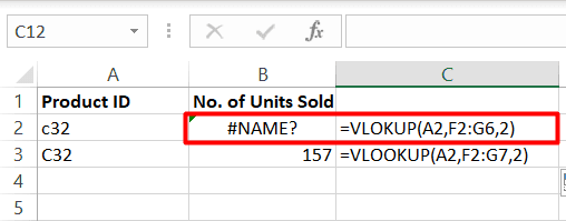

To correct this, simply replace the wrong formula name with the correct formula name.
Improper Range Usage
In case you are using range references inside your formulas, you have to be careful to avoid name errors. Any improper range reference will trigger the NAME error in Excel. For example, if you refer to the range B2 to B20 by B2B20 instead of B2:B20, Excel will show you the #NAME error.
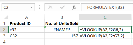

Replace all improper usage to clear the #NAME error.
Misspelled Named Ranges
Similarly, if you have accidentally misspelled a named range, expect a #NAME Excel error to show up immediately. To avoid this, correct such wrong instances and be careful while referring to them in future.


Also, be wary of using local named ranges. That is, named ranges can either be local (valid inside one worksheet only) or global (valid in all worksheets). If you accidentally refer to a local named range that is not present in your worksheet, you will face the #NAME Excel error. Use the Name Manager ( Ctrl + F3 ) to cross-check the scopes of all named ranges.


Text Not in Quotes
In Excel, when you want to refer to any text string, you have to enclose it inside two double quotes. If you don’t do this, Excel will mistake the string for a formula or a named range and will throw up a NAME error.


Also, note that you have to use the normal straight double quotes (Ex: “sample_text”) to refer to text strings. In some cases, you might accidentally use smart quotes (curly quotes), instead of straight quotes. (Ex: “right single quotation mark”). Excel will return the #NAME error since it cannot parse these smart quotes.
Keep this in mind, while referring to texts strings inside formulas.
Also Read:
How to Add Error Bars in Excel? 7 Best Methods
How to Superscript in Excel? (9 Best Methods)
Excel Goal Seek—the Easiest Guide (3 Examples)
Tip 2 – Prevent the Excel Name Error
Now that, we know how to troubleshoot each type of Excel NAME error, let us look at how to avoid them in the first place.
Take Help from Formula Suggestions
Excel has a very powerful formula suggestion feature. When you start typing in your formula after the ‘=’ symbol, Excel will automatically start suggesting suitable formulas and their respective syntaxes.
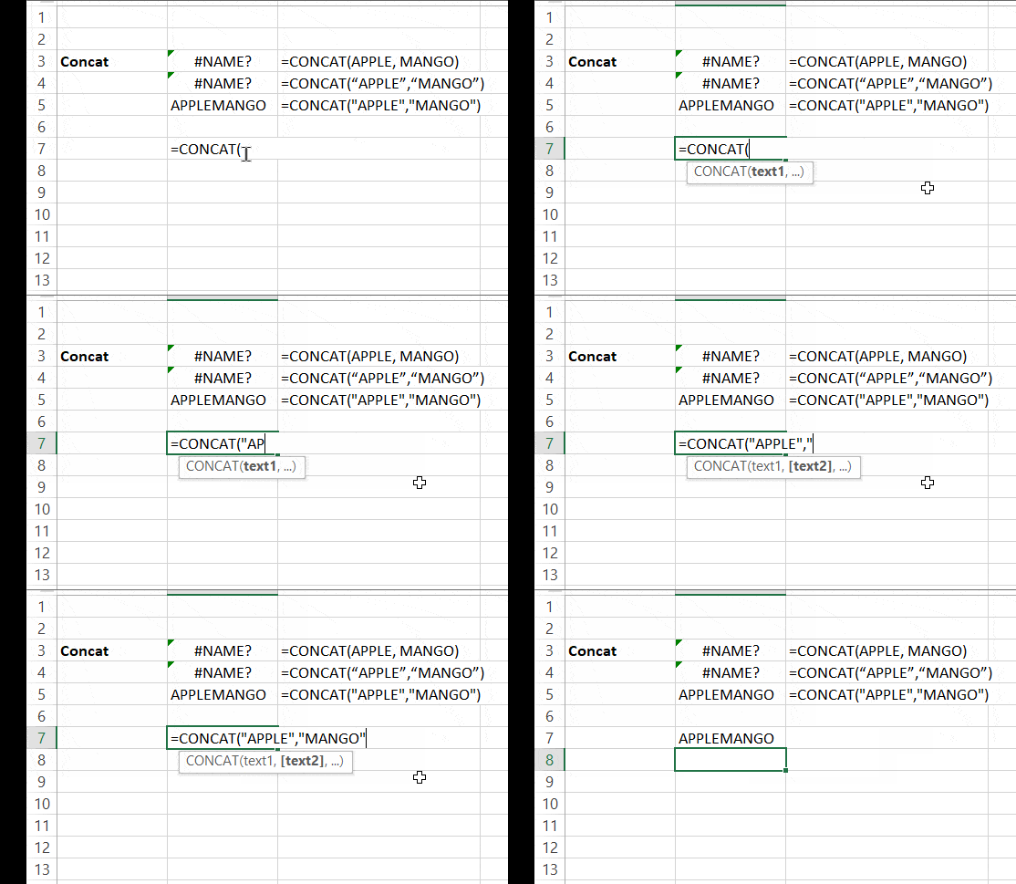

Please pay attention to these suggestions and double-check if your formulas are in accordance with the syntax.
Interestingly, if you happen to have named ranges in your sheet, these will also appear in the suggestions. This will make it easier for you to enter formulas without errors.
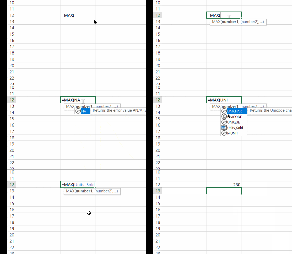

Use the Formula Wizard
Use the formula wizard, if you are still not familiar with any syntax. You can access this, by clicking on the “fx” icon right next to the formula bar.


Enter the formula name in the Insert Function box. This will take you to the function arguments dialog box, where you can enter each argument separately. Now, Excel will hold your hand and help you out in filling all the arguments.


Tip 3 – Find All the #NAME Errors in Excel
In some cases, you may want to quickly identify all the NAME errors in an Excel worksheet.
To do this, follow these steps:
- Select the data where you want to scan for errors.
- In the Home tab, click on Find & Select under the Go-to special section.


- Select, the Errors option under the Formulas section and click OK.
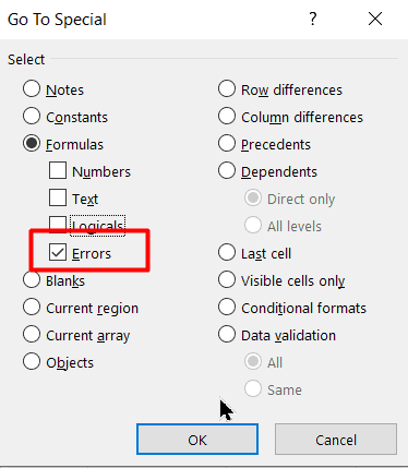

This will highlight all errors in the worksheet. Please note that this is not specific to the NAME error.


In case, you want this to be specific, follow these steps:
- Press the Ctrl+F shortcut to open the Find and Replace menu.
- Type in “#NAME?” in the Find What section
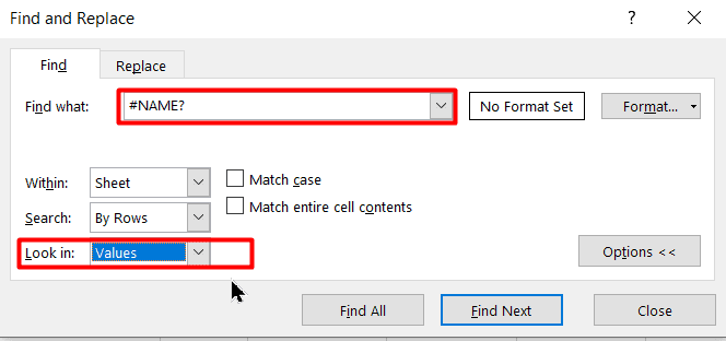

- Click on Options and set the Look In option to Values.
- Click OK.


This will list all cases of the #NAME errors and you can start resolving them one by one.
Suggested Reads:
How to Shade Every Other Row in Excel? (5 Best Methods)
How to Extract an Excel Substring? – 6 Best Methods
How to Split Cells in Excel? 3 Easy Methods
Let’s Wrap Up
That’s all folks. We hope you find this troubleshooting guide helpful. I have covered all the possible ways to fix and avoid the #NAME error in Excel. Please let us know which tip helped you the most.
To find more high-quality guides, visit our free Excel resources section.
Want to learn more about Excel? Click here to access our advanced Excel courses with in-depth training modules. You can train your entire team in Excel and other business software, for a low one-time monthly fee here.

