Getting Started with Power Pivot: Advanced Excel
Power Pivot is a tool in Excel that enables us to create data models and perform more complex operations than the standard Pivot Tables allow.
You may have seen references to the data model in Excel before when creating PivotTables – this is Power Pivot. It is also known as the data model.
This article will provide an overview of the advantages and how to get started with Power Pivot.
What are the Advantages of using Power Pivot?
Power Pivot is a data modeling tool. It prepares data for analysis in a way that has many advantages over the classic use of Excel PivotTables.
These advantages include;
Create PivotTables from multiple different tables
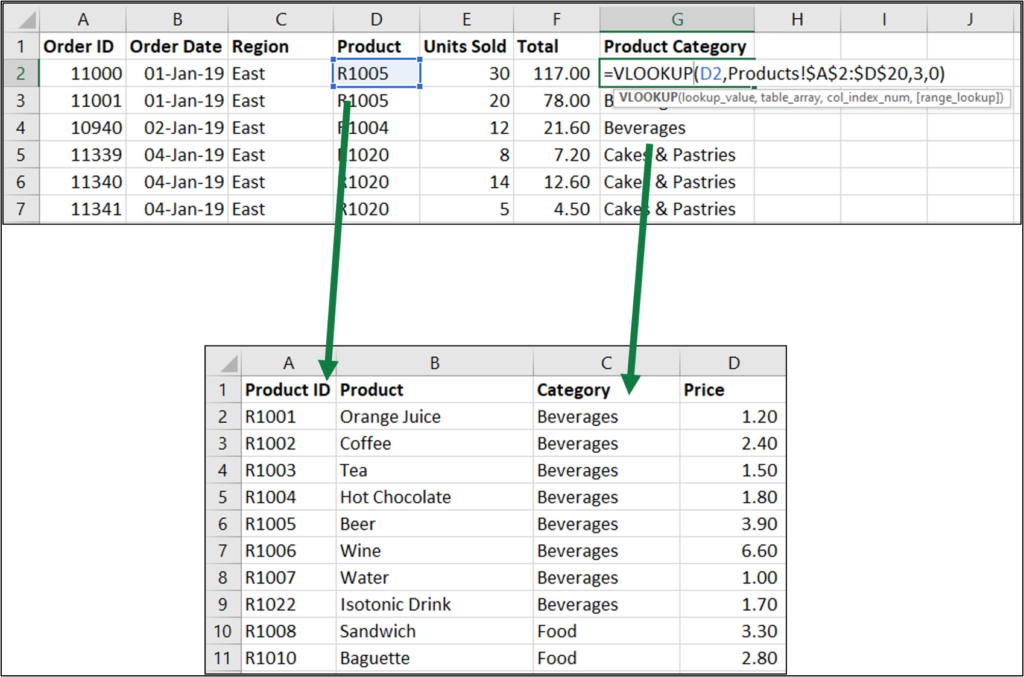
In Excel, lookup functions such as VLOOKUP are often used to combine data from multiple tables into one for a PivotTable.
In the example below, a VLOOKUP is used to return the product category from another range into a single table for a PivotTable.


With Power Pivot, you can connect to multiple data sources (Excel tables, CSV, text files, web data) and create relationships between them.
We then have a single source (the data model) to create our Pivot Tables.
In the example below, a relationship is established between the sales and products tables rather than combining the data into one.


Power Pivot can handle vast volumes of data
By connecting to external sources such as CSV files and SQL databases instead of loading the data into an Excel workbook, we can use millions of rows of data.
We are not limited by the number of rows in an Excel worksheet or constrained by the time it would take for formulas such as VLOOKUP to perform calculations.
With Power Pivot, our workbooks remain lean and fast.
More Powerful Calculations
PivotTables only provide a few calculations, such as sum, count, and average.
These are great, but if you need something different, you need to create calculated fields or write more formulas in your source data.
In Power Pivot, a formula language named DAX can be used to write formulas beyond what a standard PivotTable provides.
The aggregated formulas created using DAX are known as Measures. These Measures can be formatted in advance and are reusable in PivotTables and other Measures.
This provides a significant advantage in saving time and having faster calculations.
Getting Started with Power Pivot
Let’s walk through a simple example of using Power Pivot.
For this example, we have an Excel file with two worksheets. One with a range of sales data and the other with a range of product data.
We will load them to the data model, create a relationship between them, write some DAX formulas, and then create a PivotTable from the Power Pivot model.
Download the Excel file to follow along.
Where is Power Pivot in Excel?
There are two main ways to access Power Pivot in Excel.
You can open the Power Pivot window from the Data tab by clicking Data > Manage Data Model.
There is also a Relationships button to manage the relationships without opening the Power Pivot window.


Or from the Power Pivot tab. There is a Manage Data Model button there and also more functionality, such as being able to create Measures.


Install the Power Pivot Add-In
The Power Pivot tab is not visible by default. It needs to be installed before you can start using it.
- Click File > Options > Add-ins.
- Select COM Add-ins from the Manage list, and click Go.


3. Check the box for Microsoft Power Pivot for Excel and click Ok.


The Power Pivot tab is now available on the Ribbon. We will use this tab later in the article to create Measures.
Loading Data into the Power Pivot
In this example, we are loading data from the worksheets of this Excel file.
Let’s begin with the sales range.
- Click anywhere in the range of cells and click Data > From Table/Range.
The data needs to be formatted as a table. As this was a range, the Create Table window appears to convert the range to a table before loading it to Power Query.


The Power Query window opens. This is the tool to connect to your data sources and load them to the Power Pivot model.
2. In the Query Settings pane on the right, name the query ‘sales.’


3. On the Home tab, click the Close & Load list arrow and click Close & Load To.


4. Click Only Create Connection and Add this data to the Data Model.


This query is now loaded to the Power Pivot data model.
These steps can now be repeated for the products range. Every step is the same, except the query is named ‘products.’
The two queries are loaded to the data model and are shown in the Queries & Connections pane.


Power Query is extremely powerful and is used to get data from external sources such as Excel files, databases, CSVs, etc.
Transformation steps are performed to clean and format the data ready for the model. And these steps can be refreshed to update your reports at the click of a button.
This is a simple example to demonstrate the use of Power pivot. No Power Query steps have been used.
Take our Power Query, DAX, and Power Pivot course to see how Power Query and Power Pivot work together.
Create a Relationship between the Tables
We now need to create a relationship between the ‘sales’ and the ‘products’ tables. We can then use fields from both tables in our PivotTable reports.
Click Data > Manage data Model to open the Power Pivot window.
You are taken to the Data view. The two tables look like Excel worksheets, but they are not, and you cannot edit the cells here.
Click the Diagram View button on the Home tab.
This is the best view to create and manage the relationship between the tables of your model.
We only have two tables in this simple example. We need to create a relationship by using the two common fields, just like when using VLOOKUP to find a related match in another table.
In this example, the common fields are the ‘Products’ field in ‘sales’ and the ‘Product ID’ field in ‘products.’
Click and drag from one field to the other. As you do so, a line is drawn, and the two fields highlight green.


A one-to-many relationship has been created. A ‘1’ is shown at the end of the line by the ‘Products’ table, and an infinity symbol is shown at the end of the line by the ‘sales’ table.


Close the Power Pivot window.
Create Measures with DAX
DAX stands for Data Analysis Expressions and is the formula language of Power Pivot.
It is extremely powerful and requires much more time and demonstration than what this article can offer. Learn DAX with our Power Query, DAX, and Power Pivot online course.
As a quick example, let’s create a measure to sum the sales totals.
Click Power Pivot > Measures > New Measure


A window appears to simplify the creation of Measure and provide the options we need.
- Select ‘sales’ as the table to store the Measure in.
- Type Total Revenue for the Measure name.
- Type the following formula into the box provided. We will use a simple SUM function.
=SUM(sales[Total])
As you type a tooltip and list of tables and column names, appear to help you write the measure.


4. Select Currency from the formatting options provided. Choose which currency symbol to use and how many decimal places you want to use.


Creating PivotTables from the Data Model
We can now create a PivotTable from the data model.
The PivotTable will not look much different from any other PivotTable you have created in the past.
The name Power Pivot may be misleading in this aspect. People expect extra tools sometimes.
Power Pivot is a tool to prepare and model data ready for the PivotTable. Using the model, a PivotTable can now handle more data from multiple tables and use powerful DAX calculations.
- Click Insert > PivotTable.
- Select to Use this workbook’s Data Model.
- Choose to place the PivotTable report on a New Worksheet.


The PivotTable is inserted, and the field list shows the two tables and also the two worksheet ranges.
The two tables have a cylinder icon indicating that they are from the data model.


If we had connected data external to the workbook, we would not have seen the ranges in the worksheet.
Let’s create a quick PivotTable to see the data model and our Measure in action.
Expand the ‘products’ table and drag the ‘Category’ field to the Rows area.
Then expand the ‘sales’ table and drag the ‘Total Revenue’ measure to the Values area. The fx symbol identifies Measures.


The following PivotTable is created. It demonstrates two fields from different related tables being used, and the Measure is already formatted.


This is a simple example to show the model in operation. Go ahead and create more PivotTables and change the fields.
This article is an introduction to what is Power Pivot and a demonstration of how to use it.
To learn more enroll in our Power Pivot course
Check out a live recording of a webinar we held on Power Pivot and Power Query.
Post written by Alan Murray, founder of Computergaga

