How to Use SUMPRODUCT Function in Excel? 5 Easy Examples
(Note: This guide on how to use the SUMPRODUCT function in Excel is suitable for all Excel versions including Office 365)
The SUMPRODUCT function in Excel calculates the sum of the products of corresponding numbers in one or more ranges. It returns the sum of the products in the specified ranges of arrays. Using this function, basic mathematical operations such as addition, subtraction, multiplication, and division are possible.
The SUMPRODUCT function is categorized under Math and Trigonometry functions. This function calculates the weighted average by multiplying the corresponding components of a given array and then returning the sum of the products.
It is a handy function as it handles arrays in different ways and helps in comparing data in two or more ranges. It also helps in calculating data with multiple criteria.
In this article, I will show you how to use SUMPRODUCT function in Excel using 4 different test cases.
You’ll Learn:
- Formula
- How to Use SUMPRODUCT Function in Excel With an Example
- How to Use SUMPRODUCT Function With Matching References
- How to Use SUMPRODUCT Function With Logical Tests
- How to Use SUMPRODUCT Function to Calculate the Weighted Average
- How to Use SUMPRODUCT Function to Count the Number of Occurrences in the Table
- Few Points to Remember
Formula
| =SUMPRODUCT(array1,[array2],[array3],…) |
Parameters
Array1 – This is the first array or range that you wish to multiply and then add the products. It is a mandatory parameter.
Array2, Array 3 – These are the other arrays or ranges that you wish to multiply and subsequently add the products. These array parameters are optional.
Related Reads:
How to Use the PROPER Function in Excel? 3 Easy Examples
How to Graph a Function in Excel? 2 Easy Ways
How to Use the ROUND Function in Excel?
How to Use SUMPRODUCT Function in Excel With an Example
The SUMPRODUCT function in Excel is easy to use as any other function. Mention the cell range with the formula to get the result. Each cell in column B is multiplied by column C, and the results are added up. The total cost is $1635.
In the example above, the formula to calculate the total cost is =SUMPRODUCT(B2:B5, C2:C5).
The cells B2 are multiplied with C2 and the result is added to the result of B3* C3, and so on until the end of the range you’ve mentioned in the formula.
But, the actual formula to calculate the total cost would be =(B2*C2+B3*C3+B4*C4+B5*C5). Instead of doing it in two steps, the function SUMPRODUCT does it in one.
How to Use SUMPRODUCT Function With Matching References
In the example above, we have to check the total sales of an item in a given branch. The formula to calculate the sales is =SUMPRODUCT((A2:A9=A12)*(B2:B9=B12)*(C2:C9)). The formula first multiplies the number of occurrences of South by the number of matching occurrences of Laptop.
Then, it sums the values of the corresponding rows in the Sales column. To check how Excel calculates the formula, select the formula cell and go to Formulas -> Evaluate Formula -> Evaluate.
This formula debugs a complex formula and evaluates each part of the formula individually. Stepping through the formula part by part can help you verify whether it is calculating correctly.
When you click on the Evaluate button, it returns the result as shown below. The formula takes all the values in the first array and compares them with the condition that we have given in the formula. In this example, it takes all the values in column A and compares them with the condition ‘South’ that we have given in the formula.
How to Use SUMPRODUCT Function With Logical Tests
We can find the total sales of the product Computer irrespective of the region. To do so, use the formula =SUMPRODUCT(–(B2:B9=”Computer”),C2:C9). The reason for providing double negative (–) before mentioning the range of the cells is to force Excel to convert the TRUE and FALSE values into 0’s and 1’s.
A virtual representation of the two arrays as first processed by the SUMPRODUCT formula is shown below.
| Product | Sales in $ |
| TRUE | 2300 |
| FALSE | 1245 |
| FALSE | 3575 |
| FALSE | 1785 |
| FALSE | 2500 |
| FALSE | 2468 |
| TRUE | 8532 |
| FALSE | 1245 |
The first array contains the TRUE/FALSE values that resulted from the expression B2:B9=” Computer”, and the second array contains the values in C2:C9. The value in the first array is multiplied by the value in the second array.
If you execute the formula as =SUMPRODUCT((B2:B9=”Computer”),C2:C9), the result would be zero, as the TRUE and FALSE values will be treated as zeroes. To return the values, the values in array1 have to be numeric, so it has to be converted to 1’s and 0’s. This is the reason for introducing the double negative in the formula. This will treat the TRUE values as 1 and the FALSE values as 0.
| 1 | 2300 | 1*2300=2300 |
| 0 | 1245 | 0*1245=0 |
| 0 | 3575 | 0*3575=0 |
| 0 | 1785 | 0*1785=0 |
| 0 | 2500 | 0*2500=0 |
| 0 | 2468 | 0*2468=0 |
| 1 | 8532 | 1*8532=8532 |
| 0 | 1245 | 0*1245=0 |
The total sales are returned as 2300+8532 = 10832.
Also Read:
Battle of the Excel Lookup Functions: VLOOKUP vs INDEX/MATCH vs XLOOKUP
How to Use the Excel IFS Function? – 2 Easy Examples
How to Use the TEXTJOIN Excel Function? 3 Easy Examples
How to Use SUMPRODUCT Function to Calculate the Weighted Average
The SUMPRODUCT function in Excel calculates the weighted average where each value is assigned a weight. The weighted average takes into account the varying degrees of priority given to the numbers. Sometimes, the weighted average returns a more accurate result than a simple average.
In the example above, the weighted average is calculated using the formula, =SUMPRODUCT(B2:B5, C2:C5)/SUM(C2:C5). It first multiplies the values in the columns mentioned and then makes a sum of it. Later, to calculate the average, it is divided by the total count of items in that particular column.
How to Use SUMPRODUCT Function to Count the Number of Occurrences in the Table
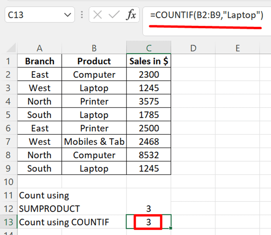
The SUMPRODUCT function in Excel can return the count of items in the table. It does the same function as that of COUNTIF and SUMIFS.
The formula, =SUMPRODUCT(–(B2:B9=”Laptop”) reduces the array values into:
–{ FALSE, TRUE, FALSE, TRUE, FALSE, FALSE, FALSE, TRUE}
The double negative converts these values to 1’s and 0’s where TRUE=1 and FALSE=0 resulting in {0,10,0,1,0,0,0,1}. The value ‘Laptop’ is an array constant and returns the value 3.
The COUNTIF function returns the number of occurrences as well. In the example below, it returns the number 3 for the search item ‘Laptop’ in the table. It returns the same result as that of the SUMPRODUCT function with double negative


Few Points to Remember
- The array that you are referencing must have the same dimensions. For example, the formula =SUMPRODUCT(B2:B5, C2:C10) will return an error #VALUE since the ranges don’t have the same size.
- SUMPRODUCT considers non-numeric values as zeros.
- Do not use the whole column’s reference with the SUMPRODUCT function. For example, =SUMPRODUCT(A:A,B:B).
- It accepts up to 255 arguments in all Excel versions from 2007 onwards.
- The function returns TRUE and FALSE values for the logical tests made within the arrays. You need to convert it into 1’s and 0’s to apply to the formula.
- It is commonly used with functions such as LEN, ISBLANK, ISTEXT, and VLOOKUP. It makes use of the result of these functions directly.
Suggested Reads:
How to Use the Excel NOW Function? 3 Examples
How to Use e in Excel Using the EXP Function? 2 Easy Examples
How to Use the Chi Square Test Excel Function? 4 Easy Steps
Closing Thoughts
The SUMPRODUCT function in Excel multiplies ranges or arrays together and returns the sum of products. This function can be used to count and sum like COUNTIFS or SUMIFS. When there is only one array, then it sums up all the values and returns them.
In this article, you learned about using the SUMPRODUCT function with different parameters. You will find these functions useful when you are making financial decisions using the data.
If you need more high-quality Excel Guides, please check out our free Excel resources center. Simon Sez IT has been teaching Excel for ten Years. For a low, monthly fee you can get access to 130+ IT training courses. Click here for advanced Excel courses with in-depth training modules.

