How to Transpose Excel Data? 2 Easy Methods
( Note: This tutorial on how to transpose Excel data is suitable for all Excel versions including Office 365. )
In Excel, transposing means switching the orientation of data from rows to columns or columns to rows. That is, it flips a vertical range into a horizontal range or vice versa.


Generally, it is used to make better sense of the data, plot graphs, do matrix operations etc. In this guide, you will learn how to transpose Excel data using different methods. I’ll cover:
- Method 1: How to Transpose Excel Data Using Paste Special?
- Method 2: How to Transpose Data in Excel Using the TRANSPOSE Function?
Related:
How to Use the NPER Excel Formula: 2 Easy Examples
The Excel SMALL Function – 3 Best Examples
The Excel CHOOSE Function – 4 Best Uses
Method 1: How to Transpose Excel Data Using Paste Special?
Paste special is the easiest way to transpose Excel data. To do this, follow these steps:
- Select the data range you want to transpose.
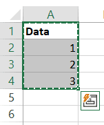

- Press Ctrl+C to copy.
- Go to the destination cell and press Ctrl+Alt+V or Alt+E+S to use paste special.


- Click on the Transpose option in the Paste Special menu and click OK. Alternatively, use the shortcut Ctrl+Alt+V+E and Enter.


Method 1.a: How to Dynamically Transpose in Excel Using Paste Special?
It is still possible to link the transposed values to their original values and make them dynamic using the Paste special feature. Here’s how:
- Copy the original values and in a different location use the shortcut Ctrl+Alt+V or Alt+E+S shortcut (paste special).
- In the Paste Special menu, choose Paste Link and click OK.


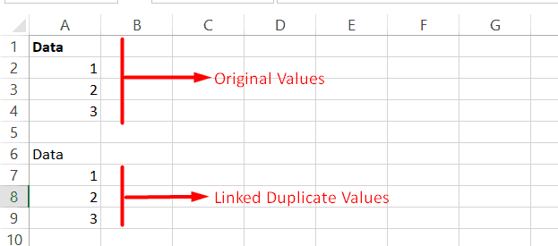

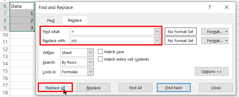
- Now, select the pasted values and press Ctrl+F to open the Replace and FInd menu. In this menu, go to the Replace tab and replace all ‘=’ with ‘yyy’ or any other character of your choice.


- Next, transpose these pasted values using the Paste Special menu as usual.
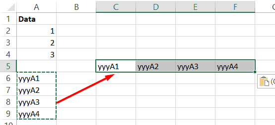

- Now, select the transposed values and press Ctrl+F to open the Find and Replace menu. In the Replace tab, replace all the ‘yyy’ to ‘=’.


That’s all. Your transposed values are successfully linked to their original values, and hence are dynamic. All changes in the original values will get reflected in the transpose.


Also Read:
How to Use Goal Seek in Excel? (3 Simple Examples)
How to Insert Multiple Rows in Excel? The 4 Best Methods
How to Autofit Excel Cells? 3 Best Methods
Method 2: How to Transpose Data in Excel Using the TRANSPOSE Function?
The TRANSPOSE formula in Excel automatically switches the orientation of ranges from rows to columns and vice versa.
To use it in older versions of Excel (2013 – 2019) follow these steps:
- Select the range of cells where the transposed data should appear. Keep in mind that, in this range, the number of columns should match the number of rows in the original data. Similarly, the number of rows should match the number of columns in the original data.


- Enter the formula =TRANSPOSE(A1:A4), wherein, A1:A4 is the original data range.
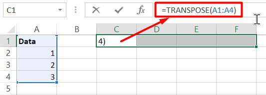

- Press Ctrl+Shift+Enter to indicate that you have entered an array formula.


That’s all, your transposed data will now appear in the designated location.
Using the TRANSPOSE function in Excel 365 is very straightforward. Just enter the formula in the first cell of the designated output location and press Enter. Since it is a dynamic array formula, Excel will automatically fill the transposed data in the nearby cells.


Method 2.a: How to use TRANSPOSE in Excel Without Converting Blanks to Zeroes?
When you use the TRANSPOSE function in Excel, it will automatically convert blanks into zeroes in the results. To avoid this, slightly modify the transpose formula to = TRANSPOSE(IF(A1:A4=””,””,A1:A4)). Using this formula will keep the blanks, as it is, in the transposed data.


Things to Keep in Mind When Using the Excel TRANSPOSE Function
The Excel TRANSPOSE function is a dynamic array formula. That is, it generates multiple results and spills over them into adjacent cells.
You can directly use it in Excel versions included in Office 365 since they support dynamic array formulas by default.
But, If you are using it in older versions of Excel, keep in mind that you have to specify the exact range size of the spill and then enter the formula. Finally, don’t forget to press Ctrl + Shift + Enter to declare it as an array formula.
Suggested Reads:
How to Group Worksheets in Excel? (In 3 Simple Steps)
How to Shade Every Other Row in Excel? (5 Best Methods)
How to Use the Excel Fill Handle Easily? (Top 3 Uses with Examples)
FAQs
What is the Excel Transpose Shortcut key?
To quickly transpose in Excel, copy the cells you need to transpose and click on the destination cell. Then use the Excel transpose shortcut Ctrl+Alt+V+E and click on Enter.
How to transpose a table in Excel?
To transpose a table in Excel, use the =TRANSPOSE(Table1[[#All],[Data]]) function in the destination cell. Replace the name of Table1 appropriately. Also, keep in mind that the transpose via paste special option is not available for tables. Hence, you need to convert a table into a normal range if you want to transpose it using Paste Special
Closing Thoughts
In this guide, we looked at the two main ways to transpose Excel data. I recommend you try these out in a practice Excel sheet to gain a better understanding. If you have any questions about this or any other Excel feature, feel free to ask in the comments section. We are always happy to help.
Want more high-quality guides for Excel? Check out our free Excel resources centre.
Click here to access in-depth Excel training courses and master in-demand advanced Excel skills.
Simon Sez IT has been teaching critical IT software for over ten years. For a low, monthly fee you can get access to 100+ IT training courses by seasoned professionals.

